Showing posts with label BMM Layer. Show all posts

Regular Expressions in OBIEE

When reporting against an OLTP system, in many ways, OBIEE works like an ETL tool, transforming the source system data and presenting it as a star schema. After years of writing ETL code, if there’s one thing I hate to be without, it’s regular expressions. So, when working on a project to map an OLTP source system to a logical model in OBIEE, I came across the following issue, and knew immediately that I would need regular expressions to solve it.
The CONTACT table in the source system had two columns storing the name: FIRST_NAME and LAST_NAME. There were two different processes that wrote entries in the CONTACT table… and one of them was faulty, writing the entire name in the FIRST_NAME column, though it was never corrected. So the following is a decent representation of what the data looked like:
SQL> create table CONTACT (contact_id NUMBER, first_name varchar2(50), last_name varchar2(50));

Table created.

Elapsed: 00:00:00.02
SQL> insert into CONTACT values (1, 'Bryson, Stewart W.', NULL);

1 row created.

Elapsed: 00:00:00.02
SQL> insert into CONTACT values (2, 'Mead, Jon', NULL);

1 row created.

Elapsed: 00:00:00.00
SQL> insert into CONTACT values (3, 'Mark', 'Rittman');

1 row created.

Elapsed: 00:00:00.00
SQL> select * from CONTACT;

CONTACT_ID | FIRST_NAME           | LAST_NAME
---------- | -------------------- | --------------------
         1 | Bryson, Stewart W.   |
         2 | Mead, Jon            |
         3 | Mark                 | Rittman

3 rows selected.

Elapsed: 00:00:00.00
SQL>
I needed to map the BMM such that I could return FIRST_NAME and LAST_NAME regardless of whether the entire name was concatenated into the FIRST_NAME, or whether it was correctly distributed across both columns. Additionally, the fact that the middle initial needed to be included with FIRST_NAME also proved a little troubling. At the end of the day, this is what I came up with in SQL:
SQL> SELECT CASE
  2           WHEN last_name IS null THEN trim(regexp_substr(first_name,'[^,]+$'))
  3           ELSE first_name
  4         END first_name,
  5         CASE
  6           WHEN last_name IS null THEN regexp_substr(first_name,'^([^,]+)')
  7           ELSE last_name
  8         END last_name
  9    FROM contact
 10  /

FIRST_NAME           | LAST_NAME
-------------------- | --------------------
Stewart W.           | Bryson
Jon                  | Mead
Mark                 | Rittman

3 rows selected.

Elapsed: 00:00:00.01
SQL>
To explain a bit, I’ll start with how I extracted the first name information from the FIRST_NAME column. I needed to start at the comma and then get the entire string until the end of the column. So I used the [^] structure in regular expressions, which basically says, return anything EXCEPT the character between the brackets and after the carrot (^). The plus (+) instructs the RegEx engine to return one or more instances of the previous structure. And at the end, the dollar sign ($) dictates that the entire string must run to the end of the column value. So taken all together, [^,]+$ instructs the RegEx engine to:
“Start at the first character that is not a comma, and return all non-comma characters all the way to the end of the column value.”
The only kludge introduced here is that the first non-comma character was actually a space, and to remove it, I simply used a TRIM. If some one has a way to do this without a TRIM, then I’d be glad to hear it.
To extract the last name information from the FIRST_NAME column, I used a similar mechanism, except that, instead of using the dollar sign ($) at the end, I put the carrot (^) at the beginning. It’s the same concept: it means that the expression returned has to begin at the start of the column value. So, the ^([^,]+ instructs the RegEx engine to:
“Start at the beginning of the column value, and return the whole string until a comma is encountered.”
Easy enough.
Now I want OBIEE to accept this SQL in the BMM. The only issue here is that OBIEE does not support regular expressions in it’s SQL language, so I have to use the EVALAUTE command to pass Oracle’s regular expression syntax back through to the database. So I’ll demonstrate how to do this, but first I’ll need to create a fact table to join to the CONTACT table in OBIEE.
SQL> CREATE TABLE activity (contact_id number, activity_date date, num_calls NUMBER);

Table created.

Elapsed: 00:00:00.04
SQL> INSERT INTO activity VALUES (1, SYSDATE-2, 10);

1 row created.

Elapsed: 00:00:00.00
SQL> INSERT INTO activity VALUES (2, SYSDATE-1, 20);

1 row created.

Elapsed: 00:00:00.00
SQL> INSERT INTO activity VALUES (3, sysdate, 30);

1 row created.

Elapsed: 00:00:00.00
SQL>
SQL> SELECT * FROM activity;

CONTACT_ID | ACTIVITY_DATE          |  NUM_CALLS
---------- | ---------------------- | ----------
         1 | 12/16/2009 10:21:34 AM |         10
         2 | 12/17/2009 10:21:34 AM |         20
         3 | 12/18/2009 10:21:34 AM |         30

3 rows selected.

Elapsed: 00:00:00.01
SQL>
To demonstrate the whole process in OBIEE, I first built the BMM to bring the data in how it is from the database:
non-regexp data.png
To generate the correct data, using the regular expressions developed above, here is how I mapped the First Name attribute:
CASE
WHEN "bidw".""."STEWART"."CONTACT"."LAST_NAME" IS NULL
  THEN  Trim(BOTH ' ' FROM Evaluate('regexp_substr(%1,''[^,]+$'')', "bidw".""."STEWART"."CONTACT"."FIRST_NAME" ))
ELSE
  "bidw".""."STEWART"."CONTACT"."FIRST_NAME"
END
first_name column mapping.png
And here is how I mapped the Last Name attribute:
CASE
WHEN "bidw".""."STEWART"."CONTACT"."LAST_NAME" IS NULL
  THEN Evaluate('regexp_substr(%1,''^[^,]+'')', "bidw".""."STEWART"."CONTACT"."FIRST_NAME" )
ELSE
  "bidw".""."STEWART"."CONTACT"."LAST_NAME"
END
last_name column mapping.png
And finally… the results:
regexp data.png

Oracle BI EE 10.1.3.4.1 – BI Server Query Parameters – Driving Tables and Parameterized Sub-Queries

Whenever BI Server is used for creating reports containing data from multiple databases, BI Server acts like a mini-database engine. It does a lot of operations itself like joins, sorts, group bys etc, everything in its own memory space. Since it acts like a database engine, it has to have certain parameters that can influence the decision making execution plan or the queries it generates. For example, for the purpose of analogy, in Oracle 9i and before the execution plan generated by the Oracle database were determined by certain rules(RBO). In 10g and above, it is based on CBO where certain statistics are maintained and they internally determine the execution plan. Along similar lines, BI Server itself depends on quite a few parameters which in turn determine the execution plan of the logical queries i.e the physical queries generated.  I have listed some of the parameters here
1. Driving Tables
2. Row Counts – Imagine this as updating the stats of a database table. This is significant in certain situations which i will cover later.
3. Number of Members in a Level (more importantly the ratio of number members across levels)
In this blog entry i will cover the concept of driving tables. In many cases when a cross-database join is performed, we might not want an equi-join to be performed between a dimension table in one database and a fact table in another database within the BI Server memory space. Instead, we might want to convert the dimension table(the column on which the join is made) into a set of literal values and then push those literal values as a filter to the fact table. That way, the queries will be constrained only to their respective databases and BI Server does not have to do any in-memory stitch joins. The diagram below explains the concept
image
As you see, all we want to do is to negate the BI Server in-memory join and convert the where clauses to individual literal filters applied directly as a physical query filter. To demonstrate this, i shall be using the standard SH schema. And to simulate multiple databases, i will model the CHANNELS dimension to be from one database and the SALES Fact to be from another database as shown below
image
Now, include these 2 tables in a BMM. But while doing a complex join between these 2 tables, enable the driving table as the Channels logical table
image
Create a simple report as shown below.
image
The above report will result in 2 queries. Both the queries are given below
select T8916.CHANNEL_CLASS as c1,
     T8916.CHANNEL_ID as c2
from
     CHANNELS T8916
order by c2
select T8924.CHANNEL_ID as c2,
     sum(T8924.AMOUNT_SOLD) as c3
from
     SALES T8924
where  ( T8924.CHANNEL_ID in (::PARAM1, ::PARAM2, ::PARAM3, ::PARAM4,
::PARAM5, ::PARAM6, ::PARAM7, ::PARAM8, ::PARAM9, ::PARAM10,
::PARAM11, ::PARAM12, ::PARAM13, ::PARAM14,
::PARAM15, ::PARAM16, ::PARAM17, ::PARAM18, ::PARAM19, ::PARAM20) )
group by T8924.CHANNEL_ID
order by c2
If you notice the 2nd query, you would notice that the CHANNEL_ID is actually converted into individual literals and then pushed as a filter. You would also notice that there are 20 such parameters. There are 2 parameters that determine the maximum number of parameters and the maximum number of queries required to generate such parameters. They are
1. MAX_PARAMETERS_PER_DRIVE_JOIN
2. MAX_QUERIES_PER_DRIVE_JOIN
Both these parameters are actually part of the database features that can be altered.
image
Just be aware that if your dimension has more members than that determined by the MAX_PARAMETERS_PER_DRIVE_JOIN, then that will throw an error. It is recommended not to use this for big dimensions as that will negate any gains we can achieve through this method. But this is very useful if you have a simple small lookup table or excel sheet somewhere that would have to act as your dimension.

BBM Layer Objects

The Business Model and Mapping layer is where physical schemas are simplified and reorganized to form the basis of the users’ view of the data. It contains the business model definitions and the mappings from logical to physical tables. The main purpose of the business model is to capture how users think about their business using their own vocabulary.
BMM Layer Objects
· There can be multiple business models in this layer.
· The business model object is the highest-level object, and it contains logical tables, logical table sources, logical columns, logical keys etc.
· Logical tables also have a Sources folder that contains one or more logical table sources. These logical table sources define the mappings between the logical table and the physical tables where the data is actually stored.
· In the Business Model and Mapping layer, data is separated and simplified into facts and dimensions.
· Business Model and Mapping layer objects map to source data objects in the Physical layer.
· Use the naming convention to re structure the model for easy understanding.

BBM Layer – Logical Table & LTS

Logical Tables
· Logical tables exist in the BMM layer and represent fact or dimension data.
· Logical fact tables have a yellow icon and logical dimension tables have a white icon.
Logical Table: Properties
· Bridge table is checked to resolve many to many relations between the tables.
· Sources tab contains the LTS, keys tab contains primary key and foreign keys tab contain foreign keys.
· You can re-order the columns in the table.
· The logical schema defined in each business model needs to contain at least two logical tables and you need to define relationships between them.
· You can create the logical tables either by dragging the physical table or manually creating it on the BMM layer.
· When you drag physical tables (with key and foreign key relationships defined) to a business model, logical keys and joins are created that mirror the keys and joins in the physical layer.
Logical Table Sources (LTS)
· Logical table sources define the mappings from a logical table to a physical table. A logical table’s Sources folder contains the logical table sources.
· Logical table source can have more than one sources from the physical layer. For example, revenue information may come from multiple data sources in a business. So, you can add these three sources to one LTS with joins. Another example could be to combine detailed level data and aggregated data, the OBI server will fetch the best source when queried on the reports.
· When you create logical tables and columns by dragging from the Physical layer, the logical table sources are generated automatically.
Logical Table Source (LTS): Properties
· Double click on the LTS to open the LTS properties screen.
· The general tab contains name other sources with join relations.
· Use the Column Mapping tab of the Logical Table Source dialog box to build, view, or modify logical to physical column mappings.
· A mapping can also be used to specify transformations that occur between the Physical layer and the Business Model and Mapping layer (Example: changing an integer data type to a character type or find a percentage of sales per unit of population.
· The Content tab is used to describe the aggregation levels (logical level or by column), to mention the fragmentation content, filter data by using where clause section and also to select distinct values.

Fact-Based Partitioning

One of the questions that comes up over and over again is how to show all periods in a query when facts don’t exist for all periods or how to show all products when facts don’t exist for all products.
To illustrate the problem, I created a database of fictional frosting sales. This is a very simple star schema having a period table, a product table, and a fact table containing weekly sales data for the last eleven weeks of 2003.
clip_image002
clip_image004
One of the frosting products, the “Party” frosting, was only introduced during the week of 11/6, however. Its sales data look like this – with nothing for the weeks in October.
clip_image006
How do you construct the metadata to show zero sales in October for Party frosting?
This is often thought of as a relational database outer join problem, which brings up another question frequently asked: how do you specify an outer join in the metadata?
Quite often, people think of this as a property of the physical join between these tables. However, if you look at the physical join properties in the metadata, you can see that the dialog does not give you any way to specify that the join should be an outer join. Notice that the join type drop down control is not active – it is grayed out.
clip_image008
When we designed OBIEE, we put control over the join type in the business model diagram because it really is a property of the business model – that is, it’s a property of the relationship between the period dimension and the facts. No matter how many period table sources or fact table sources there might be at different levels of granularity (aggregation), the join relationship should be the same within the business model.
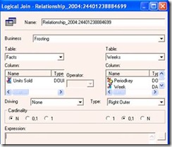
So to change the join type, use the business model diagram and change the join type between the logical tables. In the screen shot shown here, I have changed the join type to “Right Outer”. (“Right” is correct in this context since the table having the rows to preserve, the Weeks logical table, is on the right in this dialog).
clip_image010
If you examine the physical SQL after making the change, you can see the outer join being done, with the “right outer join” now translated into a “left outer join” in the SQL since the Weeks table is now “on the left” in the SQL.
SELECT T2382.DESCRIPTION AS c1,
T2388.WEEK AS c2,
sum(T2373.QS) AS c3
FROM
FROSTINGPRODUCTS T2382,
FROSTINGWEEKS T2388 left outer join
FROSTINGFACTS T2373 On T2373.PERIODKEY = T2388.PERIODKEY
WHERE
( T2373.PRODKEY = T2382.PRODKEY AND T2382.DESCRIPTION = 'Party' )
GROUP BY T2382.DESCRIPTION, T2388.WEEK
ORDER BY c1, c2
So does this solve the problem? If you look at the results, you can see that it doesn’t.
clip_image012
Perhaps you might be thinking that you might need to outer join the product table to the fact table, too. But this doesn’t give you the right results, either. Even with full outer joins, the results are still exactly the same.
This is the physical SQL generated by using full outer joins between the dimension tables and the fact table in the business model.
SELECT t2382.DESCRIPTION AS c1
,t2388.week AS c2
,SUM(t2373.qs) AS c3
FROM frostingproducts t2382
FULL OUTER JOIN (frostingweeks t2388
FULL OUTER JOIN frostingfacts t2373
ON t2373.periodkey = t2388.periodkey)
ON t2373.prodkey = t2382.prodkey
WHERE (t2382.DESCRIPTION = 'Party')
GROUP BY
t2382.DESCRIPTION
,t2388.week
ORDER BY c1,c2
It produces these results
clip_image014.
Let’s think about how to solve this problem in SQL. First calculate the sum of units sold by week for the ‘Party’ frosting. The SQL for that could look like this:
SELECT  
F.PRODKEY
,W.WEEK
,SUM(F.QS) UnitsSold
FROM    
FROSTINGWEEKS W
INNER JOIN FROSTINGFACTS F
ON F.PERIODKEY = W.PERIODKEY
WHERE    F.PRODKEY IN
(SELECT Prodkey
FROM   FROSTINGPRODUCTS
WHERE  Description = 'Party')
GROUP BY F.PRODKEY, W.WEEK


This SQL would produce the familiar results we have already seen.


clip_image016


For the next step, outer join the Products and Weeks table together without using the fact table.


Select P.Description
, P.Prodkey
, W.Week from
frostingproducts P
,frostingweeks W
where P.Description = 'Party'
clip_image018
Then left join the second result set to the first one. In terms of SQL, it would look like this:

WITH D1 AS
(select F.PRODKEY
,W.WEEK
,sum(F.QS) UnitsSold
FROM
FROSTINGWEEKS W inner join
FROSTINGFACTS F On F.PERIODKEY = W.PERIODKEY
WHERE F.PRODKEY IN (SELECT
Prodkey
FROM
FROSTINGPRODUCTS
WHERE
Description = 'Party')
GROUP BY F.PRODKEY, W.WEEK ORDER BY 2),
D2 AS
(Select P.Description, P.Prodkey, W.Week FROM
frostingproducts P
,frostingweeks W
WHERE P.Description = 'Party')
SELECT D2.Description, D2.Week, nvl(D1.UnitsSold,0) UnitsSold
FROM D2 left join D1
on D2.Prodkey = D1.Prodkey
AND D2.Week=D1.Week
ORDER BY 2
clip_image020
An OBIEE business model could be constructed to produce SQL like this. One way to do it would be to join the period and product tables into a single logical dimension table (outer joining the underlying physical tables in the logical table source), then left joining this dimension table to the logical fact table.

Here’s the physical join diagram, with the join between Products and Weeks being a complex join with the condition 1=1.


clip_image022


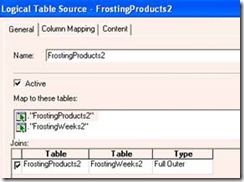
A single logical table source combines Products and Weeks.


clip_image024
The business model would contain just two logical tables and a single logical join. Note that it is a Left Outer join.
clip_image026
With this metadata, the logical SQL
SELECT Products.DESCRIPTION
, Weeks.WEEK
, FrostingFacts.UnitsSold
FROM Frosting2
WHERE Products.DESCRIPTION = 'Party'
produces this physical SQL
SELECTT2534.DESCRIPTION AS c1
, T2539.WEEK AS c2
, sum(nvl(T2526.QS , 0)) AS c3
FROM
(FROSTINGPRODUCTS T2534 /* FrostingProducts2 */
full outer join
FROSTINGWEEKS T2539 /* FrostingWeeks2 */ On 1 = 1) left outer join
FROSTINGFACTS T2526 /* FrostingFacts2 */
On T2526.PERIODKEY = T2539.PERIODKEY
AND T2526.PRODKEY = T2534.PRODKEY
WHERE
( T2534.DESCRIPTION = 'Party' )
GROUP BY T2534.DESCRIPTION, T2539.WEEK
ORDER BY c1, c2
giving the desired results.

clip_image028
(Note on the logical SQL: the columns from the single logical table “FrostingProducts2” have been separated into two presentation layer folders, “Products” and “Weeks”).
However, I don’t recommend this as a solution as you may not always want these results, but now you’ve hard-wired them into the metadata.
A better approach is to take advantage of the concept of “fact-based partitioning”. Fact-based partitioning is a term meaning that facts are stored (“partitioned”) in separate physical tables. These tables are configured as separate logical fact table sources in the metadata. When facts from two fact table sources are included in a query, the BI Server generates SQL with two query blocks and full outer joins the result sets together -- just the behavior we want.
In this case, we need to preserve both the weeks and the products and need a fact that will be returned for all weeks and products specified by the query filter.
I use a one row table to hold this fact. If you’re using Oracle as a database, you can use the virtual table “Dual”. If you’re using SQL Server, you can create a Select statement without a FROM clause to do the same thing (or you can create a one-row table in the database).
Step 1: In the physical layer create a source for the fact that will always be returned. I’ve used a Select statement to create this table:
clip_image030
Step 2: Join this table to the dimension tables with a complex join having the condition 1=1.

Step 3: Add this fact (renamed here as “PreserveDimensions”) as a new logical fact sourced from a new logical table source.

clip_image032
The fact has an aggregation rule of Max. Therefore it will always equal 1.
Step 4: Add this fact to the presentation layer.
Step 5: Create a query with a filter PreserveDimensions = 1 and save this filter. Call it “Preserve Dimensions = True”.


clip_image034


Now to preserve dimensions the user just needs to add this filter to the query. Here’s the query with just a filter on product description:


clip_image036


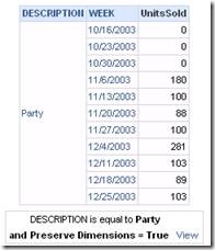
Now here’s the same query with the Preserve Dimensions filter added:


clip_image038
This query produces physical SQL that has the same form we looked at earlier. It has a query block calculating UnitsSold by Product Description and Week. It has a query block joining the Product Table and the Dimension Table, qualifying the full outer join where Description = ‘Party’.
SELECT
max(T2616.One) AS c1
, T2631.DESCRIPTION AS c2
, T2637.WEEK AS c3
FROM
FROSTINGWEEKS T2637 /* FrostingWeeksFBP */
, FROSTINGPRODUCTS T2631 /* FrostingProductsFBP */
, (SELECT 1 One FROM Dual) T2616
WHERE ( T2631.DESCRIPTION = 'Party' )
GROUP BY
T2631.DESCRIPTION
, T2637.WEEK
HAVING max(T2616.One) = 1
The SQL then outer joins the two result sets together, thereby preserving all the dimension values specified in the query filter.
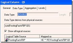
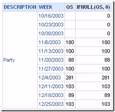
Note: to display zeros for the weeks where values are NULL, I created a logical column using the ifnull function. In the database, the actual physical column is called QS (i.e. quantity sold). The logical column QS (i.e. Quantity Sold) is mapped directly to this physical column. The logical column UnitsSold is based on the logical column QS.
clip_image040

clip_image042
Now the Answers user can choose whether to display NULLs as zeros or not by selecting the appropriate measure, as well as whether to preserve dimensions or not by clicking on the saved filter.

clip_image044
An alternative to adding the ifnull function in the metadata would be to use it in the column formula on the Criteria tab in Answers.
image
Note: on versions of OBIEE that included the Time Series functions Ago and ToDate prior to 10.1.3.3.2, this solution would have produced an error since complex joins from a period table source were not allowed. For these versions of OBIEE, the technique described here would have to be modified slightly by altering the Weeks table . Add a column to the Weeks table where all rows have the value of 1. Then join this “key” to the Dual table with a Key/Foreign Key physical join.

Two ways to define your own calculations (indicators) in the Business model

As mentioned in the article Oracle BI metadata repository - IV. Create custom indicators , there are two ways to define your own calculations (indicators), namely:

  1. Calculated on the basis of already existing logical columns(see procedure. article above)
  2. Calculation based on physical columns (procedure below)

Not matter which of the above methods you use . For each of them is generated by other physical SQL query, and in certain cases (see below) can affect the accuracy / inaccuracy of the results and even the performance itself query:
  • For calculations on the basis of already existing logical columns , first apply aggregate functions (those that are set to logical columns of which are based), and only then performs the actual calculation
  • For calculations based on physical columns is first performed to calculate and then applies the aggregate functions


An example of when to use a calculation based on physical columns 

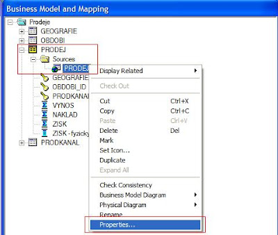
for the correct calculation of total revenues for each first row multiplied by price per unit (Unit Price) the number of units sold (Units Sold) and then only applies aggregate functions SUM (). If usethe calculation based on existing logical columns , would be erroneous calculation of total revenues . And because the first apply the aggregate function SUM () "Unit price" is 500 + 400 + 300 = 1,200 "Units sold" is 2 + 3 + 4 = 9 , and only then performs the calculation, which in this case wrong: 1.200 x 9 = 10 800 How to define the calculation based on physical columns firstSelect facts table> right click> New Object> Logical Column ... 2ndName the pointer and select OK. 3rd Choose your source physical logical table and select "Properties ..." 4th Select the Column Mapping tab (here you can see how they are mapped to each logical column from Business Model for the physical layer)> select a new pointer and start the Expression Builder (press ...) 5th In the Expression Builder, define your own calculation of the physical column and select OK 6thThe calculation is displayed in the mapping between business model and a physical layer of the 7th Finally, set an aggregate function for your new indicator and move it into the presentation layer Erik Eckhardt.