Fragmentation in OBIEE

We use fragmentation when we have fact or dimensional data in one or more different tables or data is splitted in different data sources. Then each logical table source represents one data segment.

For example, clients, in the first table are clients from A to M, in the second from M to Z.

Fragmentation of dimension

If our dimensional data is located on two or more physical tables in database (tables) or it is on separeted data sources then we can handle this by using UNION ALL views in physical layer.

However for testing this option we'll simulate this by using CHANNELS table. So we splitt it to a table CHANNELS_OTHER and CHANNELS. Fragmentation attrubur is CHANNEL_ID.


In our SALES fact table that we used here we use CHANNEL_ID from both tables CHANNELS and CHANNELS_OTHER.

Physical model, join:


SALES.CHANNEL_ID >- CHANNELS.CHANNEL_ID
SALES.CHANNEL_ID >- CHANNELS_OTHER.CHANNEL_ID

BMM:


Settings:



Test in Answers:


Result:


NQQuery.log:


We see that UNION ALL is generated.

If we choose:


NQQuery.log:


We see that the SQL is using only the second fragmented logical table source and the condition is applied only for that logical table source.

If we choose:


NQQuery.log:


If we now choose any other attribut (CHANNEL_CLASS) that is not CHANELL_ID which we used as a fragmentation key:


Then this condition is applied on both logical table sources CHANNEL and CHANNEL_OTHER:


Fragmentation of fact table

Let's split data for SALES 1998 in separate table SALES_HIST. Data from 1998 we leave in SALES.


Physical model, join:


SALES.TIME_ID >- TIMES.TIME_ID
SALES_HIST.TIME_ID >- TIMES.TIME_ID

BMM:


Settings (for a fragmentation key we choose CALENDAR_YEAR):



Test in Answers:


Result:


NQQuery.log:


If we choose:


NQQuerylog:


If we choose:


NQQuery.log:


If we now choose any other attribut (CALENDAR_MONTH_DESC) that is not CALENDAR_YEAR which we used as a fragmentation key:


Then this condition is applied on both logical table sources SALES and SALES_HIST:


In this post we showed how to combine different sources of information using fragmentation option. We see that at any moment we can see which source OBIEE takes while generating code.

Displaying duplicate values in OBIEE reports

Usually when you run a report in OBIEE it would suppress the duplicates by default and this behavior is acceptable in almost all the cases. But I recently came across a request where they wanted to display the duplicate values.

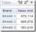
Here is screen shot of my report.

Since the Sales Amount has an aggregation rule sum defined on it, the report sums up the sale amount band groups by brand. I could display all the values for the Sales Amount by removing the aggregation rule from the measure. But this measure needs to have an aggregation rule. Or I could add some other column at the lowest grain.So here is an alternative.

Create a new column in the BMM layer (product table in this case) using an evaluate function.

EVALUATE(‘rownum’ AS INTEGER )

Adding this column in the report would display the duplicate values. You could hide the column as well.

If you get this error uncheck the pref_internal_switch_join feature in the DB features in the physical layer.

State: HY000. Code: 10058. [NQODBC] [SQL_STATE: HY000] [nQSError: 10058] A general error has occurred. [nQSError: 46030] Field descriptor id 0 is beyond the maximum field count 0. (HY000)

Using Oracle OLAP Data With Oracle BI Suite Enterprise Edition

Rit

In this example I’ll be looking at how Oracle BI Suite Enterprise Edition can be used to access data in Analytic Workspaces. Analytic Workspaces are potentially a more efficient way to store and summarize data used for reporting, as they can take up less disk space, return results faster and handle ad-hoc queries more effectively than data in traditional relational tables.

In this example, we’ll use the Global Analytic Workspace that comes with the Global Sample Schema, downloadable from OTN, and Oracle Database 10.1.2.0.2 (10.1.2.0.1 has an OLAP bug that stops it working properly, make sure you apply the patch before trying this out.) This Analytic Workspace contains a cube called “Units Cube” that is dimensioned by Product, Customer, Time and Channel.



The cube itself contains three measure; Units, Sales and Cost, and whilst some of the dimensions contain multiple hierarchies, to keep the example simple we’ll just use one hierarchy for each dimension.

Unlike OracleBI Discoverer Plus OLAP, Oracle BI Suite Enterprise Edition accesses Analytic Workspaces using SQL views over the data, rather than the Java OLAP API. When you install the Global Sample Schema using the “complete” option, the installation script creates this view for you, using the following DDL:

CREATE or REPLACE VIEW units_cube_cubeview AS SELECT *   FROM table(OLAP_TABLE('GLOBAL.GLOBAL duration session',   '',   '',   '&(UNITS_CUBE_LIMITMAP)' ))   MODEL   DIMENSION BY(       time_id,       customer_id,       product_id,       channel_id   )   MEASURES(       time_calendar_yea_parent,       time_year_id,       time_year_desc,       time_quarter_id,       time_quarter_desc,       time_month_id,       time_month_desc,       time_all_years_id,       time_all_years_desc,       time_level,       time_end_date,       time_time_span,       time_long_description,       time_short_description,       time_quarter,       time_month,       time_time_dso_1,       customer_shipments_parent,       customer_total_customer_id,       customer_total_customer_desc,       customer_region_id,       customer_region_desc,       customer_warehouse_id,       customer_warehouse_desc,       customer_ship_to_id,       customer_ship_to_desc,       customer_market_segme_parent,       customer_total_market_id,       customer_total_market_desc,       customer_market_segment_id,       customer_market_segment_desc,       customer_account_id,       customer_account_desc,       customer_level,       customer_long_description,       customer_short_description,       product_primary_parent,       product_total_product_id,       product_total_product_desc,       product_class_id,       product_class_desc,       product_family_id,       product_family_desc,       product_item_id,       product_item_desc,       product_level,       product_long_description,       product_short_description,       product_isvisible,       product_package,       product_buyer,       product_marketing_manager,       channel_primary_parent,       channel_total_channel_id,       channel_total_channel_desc,       channel_channel_id,       channel_channel_desc,       channel_level,       channel_long_description,       channel_short_description,       units,       sales,       cost,       sales_pp,       sales_chg_pp,       sales_pct_chg_pp,       sales_py,       sales_chg_py,       sales_pct_chg_py,       sales_ytd,       sales_ytd_py,       sales_ytd_chg_py,       sales_ytd_pct_chg_py,       sales_prod_prnt_share,       sales_prod_tot_share,       sales_3_per_movavg,       profit,       how_is_margin,       profit_pp,       profit_chg_pp,       profit_pct_chg_pp,       profit_py,       profit_chg_py,       profit_pct_chg_py,       profit_ytd,       profit_ytd_py,       profit_ytd_chg_py,       profit_ytd_pct_chg_py,       profit_prod_prnt_share,       profit_prod_tot_share,       profit_3_per_movavg,       olap_calc   )   RULES UPDATE SEQUENTIAL ORDER();

Note how the view uses the OLAP_TABLE function to access the analytic workspace, and the MODEL clause to improve the performance of the analytic workspace data retrieval.

Once this view has been created, you can query it in the same way as a view over a normal relational table:

SQL*Plus: Release 10.2.0.1.0 - Production on Sat Aug 5 16:34:14 2006  Copyright (c) 1982, 2005, Oracle.  All rights reserved.   Connected to: Oracle Database 10g Enterprise Edition Release 10.2.0.2.0 - Production With the Partitioning, OLAP and Data Mining options  SQL> desc units_cubeview  Name                                      Null?    Type  ----------------------------------------- -------- ----------------------------  TIME_ID                                            VARCHAR2(100)  CUSTOMER_ID                                        VARCHAR2(100)  PRODUCT_ID                                         VARCHAR2(100)  CHANNEL_ID                                         VARCHAR2(100)  TIME_CALENDAR_YEA_PARENT                           VARCHAR2(100)  TIME_YEAR_ID                                       VARCHAR2(100)  TIME_YEAR_DESC                                     VARCHAR2(100)  TIME_QUARTER_ID                                    VARCHAR2(100)  TIME_QUARTER_DESC                                  VARCHAR2(100)  TIME_MONTH_ID                                      VARCHAR2(100)  TIME_MONTH_DESC                                    VARCHAR2(100)  TIME_ALL_YEARS_ID                                  VARCHAR2(100)  TIME_ALL_YEARS_DESC                                VARCHAR2(100)  TIME_LEVEL                                         VARCHAR2(100)  TIME_END_DATE                                      DATE  TIME_TIME_SPAN                                     NUMBER  TIME_LONG_DESCRIPTION                              VARCHAR2(100)  TIME_SHORT_DESCRIPTION                             VARCHAR2(100)  TIME_QUARTER                                       VARCHAR2(100)  TIME_MONTH                                         VARCHAR2(100)  TIME_TIME_DSO_1                                    NUMBER  CUSTOMER_SHIPMENTS_PARENT                          VARCHAR2(100)  CUSTOMER_TOTAL_CUSTOMER_ID                         VARCHAR2(100)  CUSTOMER_TOTAL_CUSTOMER_DESC                       VARCHAR2(100)  CUSTOMER_REGION_ID                                 VARCHAR2(100)  CUSTOMER_REGION_DESC                               VARCHAR2(100)  CUSTOMER_WAREHOUSE_ID                              VARCHAR2(100)  CUSTOMER_WAREHOUSE_DESC                            VARCHAR2(100)  CUSTOMER_SHIP_TO_ID                                VARCHAR2(100)  CUSTOMER_SHIP_TO_DESC                              VARCHAR2(100)  CUSTOMER_MARKET_SEGME_PARENT                       VARCHAR2(100)  CUSTOMER_TOTAL_MARKET_ID                           VARCHAR2(100)  CUSTOMER_TOTAL_MARKET_DESC                         VARCHAR2(100)  CUSTOMER_MARKET_SEGMENT_ID                         VARCHAR2(100)  CUSTOMER_MARKET_SEGMENT_DESC                       VARCHAR2(100)  CUSTOMER_ACCOUNT_ID                                VARCHAR2(100)  CUSTOMER_ACCOUNT_DESC                              VARCHAR2(100)  CUSTOMER_LEVEL                                     VARCHAR2(100)  CUSTOMER_LONG_DESCRIPTION                          VARCHAR2(100)  CUSTOMER_SHORT_DESCRIPTION                         VARCHAR2(100)  PRODUCT_PRIMARY_PARENT                             VARCHAR2(100)  PRODUCT_TOTAL_PRODUCT_ID                           VARCHAR2(100)  PRODUCT_TOTAL_PRODUCT_DESC                         VARCHAR2(100)  PRODUCT_CLASS_ID                                   VARCHAR2(100)  PRODUCT_CLASS_DESC                                 VARCHAR2(100)  PRODUCT_FAMILY_ID                                  VARCHAR2(100)  PRODUCT_FAMILY_DESC                                VARCHAR2(100)  PRODUCT_ITEM_ID                                    VARCHAR2(100)  PRODUCT_ITEM_DESC                                  VARCHAR2(100)  PRODUCT_LEVEL                                      VARCHAR2(100)  PRODUCT_LONG_DESCRIPTION                           VARCHAR2(100)  PRODUCT_SHORT_DESCRIPTION                          VARCHAR2(100)  PRODUCT_ISVISIBLE                                  NUMBER  PRODUCT_PACKAGE                                    VARCHAR2(100)  PRODUCT_BUYER                                      VARCHAR2(100)  PRODUCT_MARKETING_MANAGER                          VARCHAR2(100)  CHANNEL_PRIMARY_PARENT                             VARCHAR2(100)  CHANNEL_TOTAL_CHANNEL_ID                           VARCHAR2(100)  CHANNEL_TOTAL_CHANNEL_DESC                         VARCHAR2(100)  CHANNEL_CHANNEL_ID                                 VARCHAR2(100)  CHANNEL_CHANNEL_DESC                               VARCHAR2(100)  CHANNEL_LEVEL                                      VARCHAR2(100)  CHANNEL_LONG_DESCRIPTION                           VARCHAR2(100)  CHANNEL_SHORT_DESCRIPTION                          VARCHAR2(100)  UNITS                                              NUMBER  SALES                                              NUMBER  COST                                               NUMBER  SALES_PP                                           NUMBER  SALES_CHG_PP                                       NUMBER  SALES_PCT_CHG_PP                                   NUMBER  SALES_PY                                           NUMBER  SALES_CHG_PY                                       NUMBER  SALES_PCT_CHG_PY                                   NUMBER  SALES_YTD                                          NUMBER  SALES_YTD_PY                                       NUMBER  SALES_YTD_CHG_PY                                   NUMBER  SALES_YTD_PCT_CHG_PY                               NUMBER  SALES_PROD_PRNT_SHARE                              NUMBER  SALES_PROD_TOT_SHARE                               NUMBER  SALES_3_PER_MOVAVG                                 NUMBER  PROFIT                                             NUMBER  HOW_IS_MARGIN                                      VARCHAR2(100)  PROFIT_PP                                          NUMBER  PROFIT_CHG_PP                                      NUMBER  PROFIT_PCT_CHG_PP                                  NUMBER  PROFIT_PY                                          NUMBER  PROFIT_CHG_PY                                      NUMBER  PROFIT_PCT_CHG_PY                                  NUMBER  PROFIT_YTD                                         NUMBER  PROFIT_YTD_PY                                      NUMBER  PROFIT_YTD_CHG_PY                                  NUMBER  PROFIT_YTD_PCT_CHG_PY                              NUMBER  PROFIT_PROD_PRNT_SHARE                             NUMBER  PROFIT_PROD_TOT_SHARE                              NUMBER  PROFIT_3_PER_MOVAVG                                NUMBER  OLAP_CALC                                          RAW(16)  SQL>

Notice how this particular view returns both the measures in the Units Cube, and all of the dimension member, attribute and level information from the dimensions that it references. Whilst you can create views individually over dimensions in an analytic workspace, in this example we’ll create just the one, denormalized view over all of the objects, and use BI Suite Enterprise Edition to present them to the user as separate objects. I’ll come on to ‘why’ later on in the example.

Now that I have created a view over the analytic workspace, I can go into the Administrator application and import it into the Physical Layer of the Semantic Model.



Now that I’ve brought the denormalized view into the Physical Layer, I can move on to the Business Layer to define my logical facts and dimensions.

When you work with the Business Layer of the Semantic Model, the objects you create are logical objects; logical tables, dimensions and so on. In a simple setup, your logical tables usually map one-to-one with the physical tables in your data source, but in our case we want to use the Business Layer to define logical dimensions, facts and measures based off of the single, denormalized view over our analytic workspace. That way, we only retrieve the data once, there are no physical joins taking place at the database level, and we can use the full power of the OLAP Option to process and manipulate our data.

To start off, I want to create a logical “Product” table upon which I will build a Product dimension. I create the logical Product table, and define a source for it, which I call “Item”.



I then add five logical columns to this source, four of which I map to columns on the Units_Cubeview physical table, and one of which I set to the scalar (literal) value “ITEM”.

I then add three more sources to the logical table, corresponding to the four levels (Item, Family, Class and Total Product) in the hierarchy. In these cases though, I only add columns to represent the levels upwards from the one in question, like this:



So why set the logical table up like this? Well, if you take a look back at the single denormalized view over the Units Cube, and if you took a look at the data within it, you’ll know that the cube is a “solved cube” – that is, it contains both detail level and aggregate level data in the same cube. To access aggregated data, you select against the the dimension-related columns in the cube view using the required level – in the first case, “ITEM”, in the second “CLASS”, and rely on the Oracle OLAP engine to provide the aggregation, rather than have Oracle do it using GROUP BY and SUM().

The PRODUCT_LEVEL column in each data source tells Oracle what level of aggregation to refer to; the four separate logical table sources gives the Oracle BI Server a separate complete table source for each level of the dimension hierarchy, complete with the values for that level and the ones above. When the Oracle BI Server parses your logical SQL query and works out what physical SQL it needs to generate, it will pick the appropriate table source for your level of aggregation and direct the query as appropriate. Make sure that you list the dimensions from most aggregated to least, top to bottom, as the BI Server will start at the top of the list and work down when looking for a table source with the required level of granularity.

Once I’ve worked through the Product, Customer, Time and Channel dimensions, I define the Units fact table using just a single logical table source, the Units_Cubeview I used for the dimension logical tables earlier. This time I don’t need to define more than one source for the table – this was only because I needed to create a source for each level of the dimensions – and I bring in all of the measures, plus the dimname_LEVEL columns so that the BI Server can retrieve data at the correct level of aggregation.



I’ve now completed the first part of the execise, to create some logical tables out of the single denormalized view over the analytic workspace.

The next step is to create the dimension objects in the Business Layer. Dimension objects in BI Suite Enterprise Edition define drill paths and aggregations, and I can go ahead and create them just as I would over normal, relational tables. For example, to define the Product dimension, I go ahead and create Total Product, Family, Class and Item levels, and then drag the relevant description columns from the Product logical table to create the keys.



To finish this step off, I go and create dimension objects for the other three dimensions.

Now comes the final step. We are going to use a feature in the BI Server, not unlike Virtual Private Database in the Oracle database, to append additional conditions to the ‘WHERE’ clause in order to leverage the aggregations in our analytic workspace. To do this, I create a group called “AW” using the Security Manager, like this:



and then add a security filter for each dimension table, that refers to the dimname_LEVEL column in each logical table and ensures we pick up data for the correct level of aggregation within each dimension. When it comes to retrieving data from the analytic workspace, the BI Server will now simply select the “cells” or “rows” it wants from the aggregate data, without having to worry about performing the aggregation itself.



The actual filter is defined as thus (note that the exact same filter that gets applied to each logical table):

"Global Electronics".Channel.CHANNEL_LEVEL = "Global Electronics"."Sales Fact".CHANNEL_LEVEL AND  "Global Electronics".Product.PRODUCT_LEVEL = "Global Electronics"."Sales Fact".PRODUCT_LEVEL AND  "Global Electronics".Market.CUSTOMER_LEVEL = "Global Electronics"."Sales Fact".CUSTOMER_LEVEL AND   "Global Electronics"."Time".TIME_LEVEL = "Global Electronics"."Sales Fact".TIME_LEVEL

Now, I finally need to make sure that each user who will access this OLAP data is part of the AW group, and then I can log in to OracleBI Answers and start querying my Analytic Workspace.

First of all I add the Product Class to my request, and then click on “Software/Other” to drill down to Product Family.



Taking a look at the logical SQL that Answers generates, it looks like this:



Looking the query log though, this translates into the following physical SQL, written against the Units_Cubeview view:

select distinct D1.c1 as c1,      D1.c2 as c2 from       (select distinct T4514.PRODUCT_CLASS_DESC as c1,                T4514.PRODUCT_FAMILY_DESC as c2           from                 UNITS_CUBEVIEW T4514           where  ( T4514.PRODUCT_LEVEL = 'FAMILY' and                     T4514.TIME_LEVEL = 'ALL_YEARS' and                     T4514.CHANNEL_LEVEL = 'TOTAL_CHANNEL' and                     T4514.CUSTOMER_LEVEL = 'TOTAL_MARKET' and                     T4514.PRODUCT_CLASS_DESC = 'Software/Other' )       ) D1 order by c1, c2

Now, if I add the Customer dimension, and one of the measures, into the query, I can see it working with a pivot table query:



Again, checking out the physical SQL sent to the Oracle database, you can see how it’s querying the single Units_Cubeview denormalized view over the Analytic Workspace:

select distinct D1.c2 as c1,      D1.c3 as c2,      D1.c1 as c3,      D1.c4 as c4 from       (select sum(T4514.UNITS) as c1,                T4514.PRODUCT_CLASS_DESC as c2,                T4514.PRODUCT_FAMILY_DESC as c3,                T4514.CUSTOMER_MARKET_SEGMENT_DESC as c4           from                 UNITS_CUBEVIEW T4514           where  ( T4514.PRODUCT_LEVEL = 'FAMILY' and                     T4514.TIME_LEVEL = 'ALL_YEARS' and                     T4514.CHANNEL_LEVEL = 'TOTAL_CHANNEL' and                     T4514.CUSTOMER_LEVEL = 'MARKET_SEGMENT' and                     T4514.PRODUCT_CLASS_DESC = 'Software/Other' )            group by T4514.CUSTOMER_MARKET_SEGMENT_DESC,                     T4514.PRODUCT_CLASS_DESC,                     T4514.PRODUCT_FAMILY_DESC      ) D1 order by c1, c2, c4

So, now that it’s possible, why would you want to go down this route and put your data into an analytic workspace before using it with BI Suite Enterprise Edition? Well, it comes down to two key advantages.

Firstly, the OLAP engine presents data to the BI Server as fully aggregated even if some of the totals are calculated on-the-fly, making aggregate navigation simpler and not subject to the vagaries of query optimization, materialized views and query rewrite, and also giving you the potential to completely pre-summarize your data and store these summaries right alongside your detail-level data.

Secondly, you gain access to the OLAP calculation engine, which on the one hand makes setting up standard analytic queries as simple as using a point-and-click interface (Analytic Workspace Manager), whilst on the other gives you access to high-end forecasting, allocation and statistical functions that just aren’t present in regular SQL. Once you have set up the view over your analytic workspace and created the Business Layer metadata, users won’t even know that your data is stored multi-dimensionally, all they’ll notice is a bunch of new calculations and a consistently fast response time. Finally, the OLAP engine evaluates and processes these calculations extremely fast – no joins are needed, just simple array lookups, so you are doing the calculations where they should be done – in the database using an industrial strength calculation engine.

Thanks to Marty Gubar over on the OLAP Product Management team for showing me this methodology, and keep an eye on OTN where there’ll soon be a white paper going into more details on how this is set up.

inShare