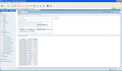
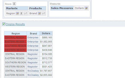
Use this approach only if you have no other options. Also, this would work only if you have non-numeric columns(on which you want to apply conditional formatting). Not an elegant solution but would work neverthless. As the title of this blog suggests we shall be looking at an approach to enable cross column conditional formatting on Pivot Tables. You might probably be aware of the fact that BI EE does not support cross column conditional formatting in Pivot Tables. This is stated very clearly in the New Features Guide here. But what if your end user somehow wants this feature. In such a case, just follow the below mentioned procedure. Lets start with a simple Pivot table report as shown below
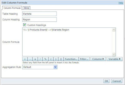
The above report gives a report on the Region, Brand and their corresponding sales. Now, our aim is to highlight all the Regions in Red whose Brand value is Enterprise. In a tabular view this is straightforward since it supports cross column conditional formatting. But since in our case this is a pivot table, go back to the criteria tab and edit the formula tab of the Region column. Type in the below formula.
‘<!– ‘|| Products.Brand||’ –>’||Markets.Region
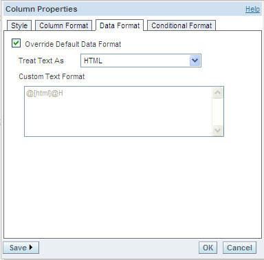
Now, convert this column to a HTML format.
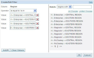
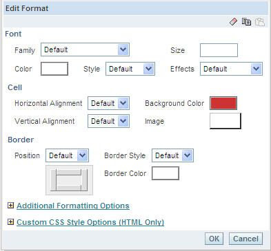
Once this is done, go to conditional format of this column and give the necessary conditional formats (You would have to choose all the 4 Enterprise Brands||Regions. This is the main drawback with this approach. It would really nice if conditional Formatting supports the containsAny operator ).
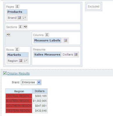
Now, if you go to the pivot table you would notice that all the regions which are under the Enterprise Brand would be highlighted. The idea is to basically concatenate the columns and then apply the conditional formatting. The formula above (which is nothing but HTML commenting) will avoid the display of the columns multiple times.
Not the best solution but can be useful if you somehow need to use cross-column formatting in pivot tables.
